
![]() By John Avina*
By John Avina*
Abstract
The Option C Measurement and Verification methods for energy service companies (ESCOs) often involve performing regressions of utility bills against weather data. We have been advised by the International Performance Measurement and Verification Protocol (IPMVP) that our regressions should yield CV(RMSE)s (coefficients of variation of the root mean square of the error), below a certain level in order for the regression to be considered statistically significant. But what happens if you have a large portfolio, such as a school district? Is it necessary that every meters’ regression have a CV(RMSE) conforming to this rule? This paper suggests that individual meters’ CV(RMSE)s do not matter. What matters is the portfolio’s overall CV(RMSE). We tested this theory on a sample of 236 meters and found that the CV(RMSE) of the portfolio can be more than 50% lower than the average CV(RMSE) of the individual meters.
Background
In previous papers, I have questioned whether the CV(RMSE) and the coefficient of determination (R2) are useful indicators of whether a regression model (or fit) is statistically significant. The general consensus of the experts is that the R2 value should be ignored, and the CV(RMSE) should be lower than a threshold for a fit to be considered acceptable.
A simplified, but not entirely accurate, definition of the CV(RMSE)1 is that it is a measure of scatter around a regression fit line. A CV(RMSE) of 10% means the average distance between a point and the fit line is 10% of the fit line.
EVO (Efficiency Valuation Organization) recommends that linear regressions have a CV(RMSE) that is less than one half of the expected savings fraction. In other words, if you expect to save 25% of the total energy usage of a meter, then your CV(RMSE) should be 12.5% or less.
The American Society of Heating, Refrigeration, and Air-Conditioning Engineers (ASHRAE) produced Guideline 14 that recommended that linear regressions having CV(RMSE) values less than 25% are acceptable.2,3
In the past I have questioned using CV(RMSE) as a means of deciding whether a linear regression model is acceptable to use or not. Recently, Professor Eric Mazzi wrote that many in the statistics community are starting to question the value of R2 and CV(RMSE) as measures to determine whether to use a regression model or not. “Statistically significant” is becoming an outmoded term.4 So, perhaps I am not alone on this point after all. It appears others are realizing this as well.
Regardless, in this article, I will assume that EVO’s the CV(RMSE) guidance holds, and we want the CV(RMSE) to be less than or equal to half the expected savings fraction.
Purpose of the Paper
Instead of challenging the appropriateness of using CV(RMSE) to determine whether a fit is statistically significant, we want instead to point out that in cases where there is a portfolio of meters, holding each individual meter to the CV(RMSE) standard may not be necessary at all.
To address this problem, I took a large data set and calculated CV(RMSE)s at the meter level and at the portfolio level and compared the two.
My Data
Having worked in utility bill analysis for over 25 years, I have some large data sets of monthly bills. In the past, I was blessed with tracking several big box store chains, one of which had 2500 meters. We performed regressions on all of these meters and estimated energy savings for our clients.
In particular, I have a data set of electricity meters for the now defunct Circuit City stores in the Eastern half of the United States. There are 263 meters in this data set.
Years ago, we performed regressions on the meter data versus cooling degree days (CDD). We deselected some outliers, many of which were estimated/actual bills.5,6 I have since then reincluded all of the outliers, so that I could have some bad fits in my data set. The worst fit in the group was for the Midlothian Virginia store. The fit provided me with a CV(RMSE) of 22.2% and an R2 of 0.227. Let’s take a look at this meter. It would actually be a good fit if I wouldn’t have reinserted the estimated and actual bills back into the regression. In Figure 1, you can see the estimated bill is well below the fit line and the actual bill, well above it. Estimated actual bills compromise the quality of fits, decreasing R2 values and increasing CV(RMSE)s.
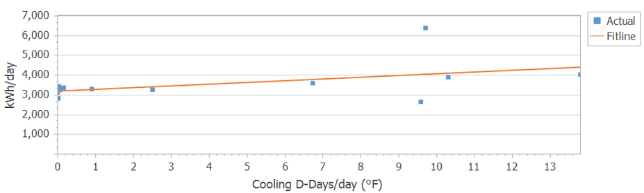
Figure 1. Linear Regression of Midlothian, VA store kWh/day vs. CDD/day.
In Figure 2, the blue dots represent bills, and the red line is what the regression equation predicts that the bills should be, based on the regression equation. You can see that the estimated bill is in June and the actual bill in July.
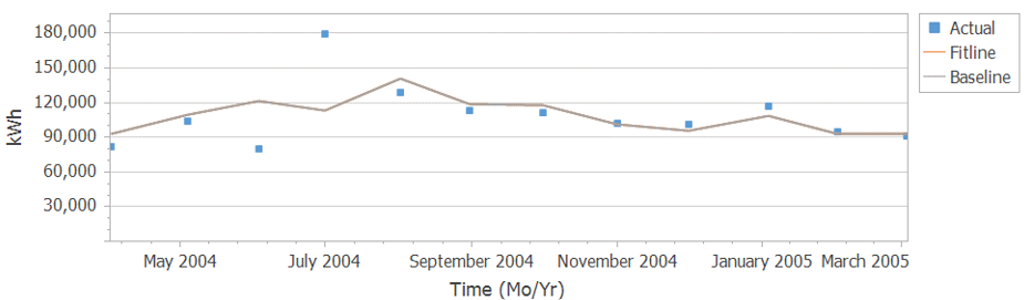
Figure 2. Linear Regression results of Midlothian, VA store kWh/day vs. CDD/day presented as kWh vs. time.
Overall Nature of Data
On average, as evidenced by the low CV(RMSE) values and the high R2 values, the regressions were of high quality, better than you would expect. I suppose that implies that the building controls worked fairly well. In other words, the building responds in a predictable manner to weather conditions.
The average R2 value of the 238 meters is 0.78, with a standard deviation of 0.20. The average CV(RMSE) of the 238 meters is 5.2%, with a standard deviation of 3.0%. Figures 3 and 4 present histograms to give you an idea of the spread of CV(RMSEs) and R2 values. The horizontal lines represent the average values.
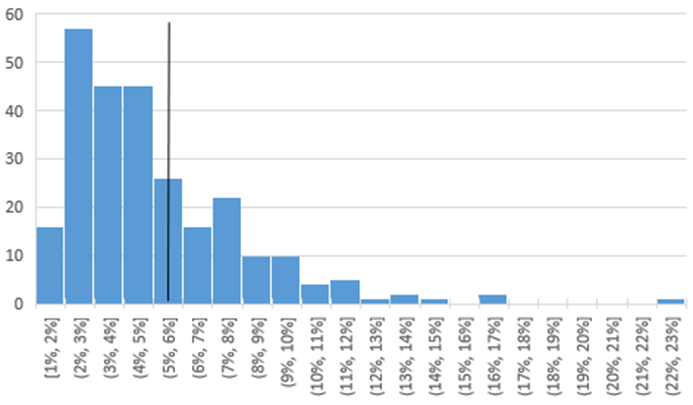
Figure 3. Histogram of CV(RMSE) from the regressions of kWh/day vs. CDD/day of all 238 stores.
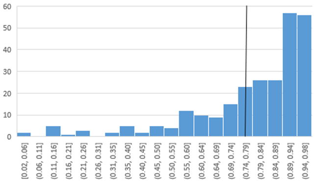
Figure 4. Histogram of R2 from the regressions of kWh/day vs. CDD/day of all 238 stores.
My Experiment
The purpose of this experiment was to determine to what extent the CV(RMSE) of the entire portfolio was different than the average CV(RMSE) of the individual meters. And how does the number of meters in the sample affect the portfolio CV(RMSE)?
I had 235 regression equations, their associated CV(RMSE)s and R2 values. For each of the 12 months in the base year period I had 235 actual bills and 235 adjusted baselines (which is what the regression equation predicts the usage should have been). Table 1 presents a snippet of actual bill data for a small number of meters. For the sake of space, I did not show all 12 months.
Table 1. A Few Months of Sample Actual Bill Data for the Base Year Period

For each month in the base year period, I summed the actual bills and adjusted baselines. The sums are presented in Table 2. Again, I only showed a few months due to space limitations.
Table 2. A Few Months Summation of All Data for 235 Meters for the Baseline Period

I calculated CV(RMSE) of this summation. I called it the Portfolio CV(RMSE).
I then started removing meters from the sample. I repeated this calculation of Portfolio CV(RMSE) for the first 200 meters, the first 150 meters, the first 100 meters, on down to the first 2 meters. Table 3, presents the results, along with average R2 values.
Table 3. Trial 1: Meters, Average R2, Average CV(RMSE), Portfolio CV(RMSE), and Reduction in CV(RMSE)

To a degree, these results were due to the particular order of the meters listed. For example, the meters with the lowest CV(RMSE) could have been the first ones I eliminated, leaving the higher CV(RMSE) meters. This could unfairly bias the results. To avoid this problem, I repeated this procedure four times. For each of these trials, I mixed the order of the meters.7
Results
For all 235 meters, we found that the CV(RMSE) dropped from 5.3% (the average of the individual meters) to 1.6% (the CV(RMSE) of the portfolio as a whole), a 70% improvement. In the first trial, in order to see a 50% improvement in CV(RMSE), we would need the portfolio to include about 17 meters. In the other trials, to get to a 50% improvement in CV(RMSE), we would need to have about 4, 8 and 20 meters. This is all shown in Table 4, which presents the reduction of portfolio CV(RMSE) from the average individual CV(RMSE).
We calculated the reduction in CV(RMSE) as follows.
Reduction % = (Average Meter CV(RMSE) – Portfolio CV(RMSE)) / Average Meter CV(RMSE)
Table 4. Reduction in CV(RMSE) from Average (CVRMSE) for All 4 Trials Using Weather Normalization

The trends are clearer in the graphical representation, as shown in Figure 5. The thick line with no markers represents the average of the four trials.
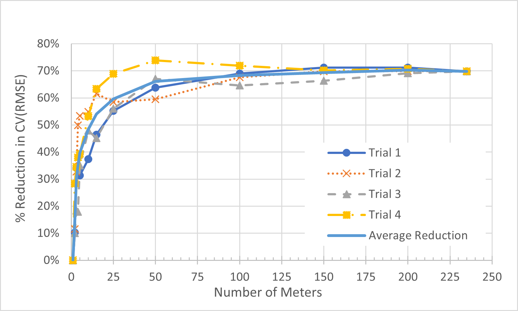
Figure 5. Percent Reduction in CV(RMSE) from Average (CVRMSE) vs. Number of Meters in Portfolio for All 4 Trials Using Weather Normalization.
Figure 6 presents the data at the lower range, because that is where it is more interesting. On average, it took about 11 meters to drop the CV(RMSE) by 50%, and 25 meters to drop the CV(RMSE) by 60%.
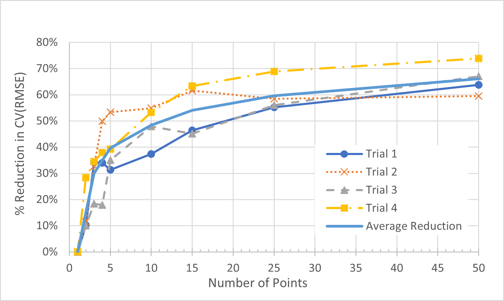
Figure 6. Percent Reduction in CV(RMSE) from Average (CVRMSE) vs. Number of Meters (for up to 50 meters) in Portfolio for All 4 Trials Using Weather Normalization.
Although we are using the same data, the meters are mixed up in different orders, so each trial effectively represents a different data set. The trials provide different results because the meters in each collection of X meters are different in the different trials. Although every data set will provide different results, we can make a generalization.
It is clear that the CV(RMSE) of the portfolio will be much lower than the average CV(RMSE) of the individual meters. A 50% reduction in CV(RMSE) is likely. But just how many meters is required to see a 50% drop in CV(RMSE)? That will depend on your data set.
Why Does the Portfolio Drop the CV(RMSE)?
The reason more meters tend to dampen the CV(RMSE) is that the randomness in the bills tends to smooth out as more meters are added to the sample. But this is not always the case.
Are there Exceptions?
Suppose you have a portfolio of 100 schools all of which use electricity to cool. Suppose you didn’t do a regression at all for these meters, and instead used an average kWh/day to represent baseline energy usage. Over the course of a year, it would even out. The kWh/day model will end up with the same number of kWh as the summation of the bills over the course of a year. The mean bias error would be 0. But on a monthly basis, the average kWh/day model would estimate low usage in summer and high usage in winter. Figure 7 represents this concept pictorially. The “fit line” represents the kWh/day model’s prediction of the monthly amounts.
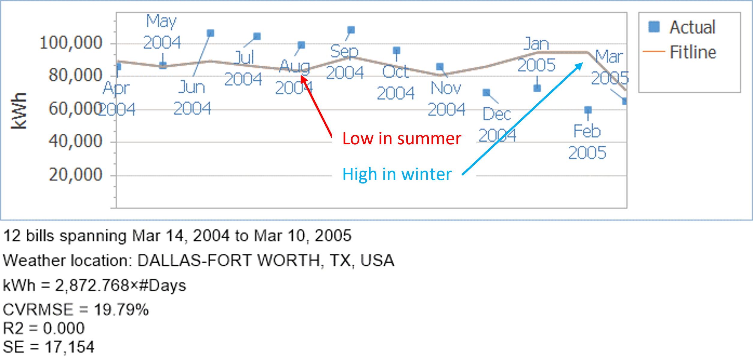
Figure 7. Average kWh/day model (fit line) prediction of monthly usage versus actual monthly usage.
What would happen if we didn’t do regressions on any of the meters in our Circuit City sample and then performed the same test?
Would the CV(RMSE)s drop, as they did in our other example?
To save time, I didn’t use all 235 meters. Instead, I took the 61 stores whose names started with an “A”, “B”, or “C.” Like before I randomized the order of the meters and took 4 trials, comparing average individual CV(RMSE) with portfolio CV(RMSE). Table 5 and Figure 8 presents the reduction of portfolio CV(RMSE) from the average individual CV(RMSE).
Table 5. Reduction in CV(RMSE) from Average (CVRMSE) for All 4 Trials Using Average kWh/Day Model.

Note: In Trial 1 of the average kWh/day models, we saw some high reductions in CV(RMSE) when the samples had 3 to 7 meters. This was due to a couple of meters having very low CV(RMSE)s. This aberrant behavior only reinforces the idea that the magnitude of CV(RMSE) reduction has much to do with the characteristics of the individual meters’ fits.
The average CV(RMSE) of these 61 stores was 12.8%. I then calculated the CV(RMSE) of the entire portfolio of the 61 stores, and got 11.2%, a reduction of only 12%. Compare that to my earlier trials. When I performed linear regressions of kWh/day versus CDD/day, at 50 meters, I had an average reduction in CV(RMSE) of 66%. That is a big difference.
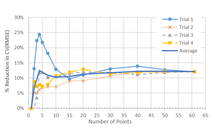
Figure 8. Percent Reduction in CV(RMSE) from Average (CVRMSE) vs. Number of Meters in Portfolio for All 4 Trials Using an Average kWh/day Model (as Opposed to Weather Normalization).
As before, there is variation in the average meters’ CV(RMSE) and the Portfolio CV(RMSE), depending on which meters are in the sample. However, overall, on average, it is clear that the measuring CV(RMSE)s at a portfolio level drops the CV(RMSE), but in this case, the CV(RMSE) did not drop by much.
So why did the CV(RMSE) of the portfolio not drop substantially in this case when I didn’t do regressions to weather?
If a regression is perfect, that is, all points are on the line, the CV(RMSE) would be zero. In our regressions, we found good fit lines, high in the summer, low in the winter, just like the bills. Because there was so little scatter, our CV(RMSE)s were low.
When we didn’t do a regression and just took the average kWh/day, we expected high CV(RMSE)s because the fit line was much higher than the winter bills and much lower than the summer bills. There was always going to be scatter. By combining the un-regressed meters together, we may have smoothed some of the scatter (hence the 12% reduction in CV(RMSE). But the general tendency of overestimating usage in the winter and underestimating usage in the summer was only reinforced because all of the meters had this same pattern. The summation of the average kWh/day models still overestimated usage in the winter and underestimated usage in the summer, which leads to higher scatter and thus higher CV(RMSE) at the portfolio level.
Conclusions
The IPMVP is suggesting that when using regression analysis as part of the Option C M&V process, the CV(RMSE) for each meter should be less than 50% of the expected savings fraction. In other words, if you expect to save 20% on a meter, then the CV(RMSE) should be less than 10%.
When performing regressions on a portfolio of buildings, such as a school district, the CV(RMSE) of each individual meter may not be that important. What perhaps may be more important is the CV(RMSE) of the portfolio of meters, which will likely be much lower than the CV(RMSE) of the individual meters.
For ESCOs performing Option C M&V on a school district, a military base, or another portfolio of meters, then perhaps the overall portfolio CV(RMSE) should be considered, rather than the CV(RMSE) of each meter. That would allow the M&V practitioner more latitude to include regressions with poor fits in the portfolio.
Ideally, the ESCO would calculate the CV(RMSE) of the portfolio and use that to evaluate the reasonableness of the collection of regression models.
This is not an original idea. CalTRACK, a collaboration of M&V specialists developed a set of guidelines for utilities when using Option C M&V methods.8 CalTRACK was well aware of the fact that CV(RMSE)s drop at the portfolio level. Caltrack has recommended that CV(RMSE)s of individual meters in a portfolio could be as high as 100%. That means, in my sloppy lay language, that the average point could be 100% away from the fit line. That is a remarkably low bar to overcome!
We are not suggesting adopting the 100% rule. Rather, the CV(RMSE) should be evaluated at the portfolio level and not at the meter level.
NOTES:
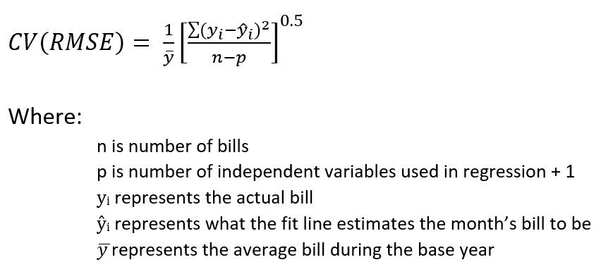
[1] The official definition of CV(RMSE) is:
[2] Actually, ASHRAE 14-2014 says: “the baseline model shall have a maximum CV(RMSE) of 20% for energy use and 30% for demand quantities when less than 12 months’ worth of post-retrofit data are available for computing savings. These requirements are 25% and 35%, respectively, when 12 to 60 months of data will be used in computing savings. When more than 60 months of data will be available, these requirements are 30% and 40%, respectively.”
[3] ASHRAE 14 also requires that the fractional savings uncertainty (FSU) be less than 50 % of the annual savings at 68 % confidence.
[4] Mazzi, Eric, “Commentary on Article ‘Statistics and Reality—Addressing the Inherent Flaws of Statistical Methods Used in Measurement and Verification’”, International Journal of Energy Management, Volume 4, Issue 2, 2022
[5] Estimated/Actual refers to cases where the utility does not read a meter one month, and instead estimates what the bill should be. Invariably, this “estimated” bill is low. They then follow that bill up, the next month, with an “actual” bill, which is a real reading, but is high, as it contains the second month’s usage plus the underage from the first month.
[6] I know, there are better ways to handle this. Today, I would combine the two bills into one, and then the combined bill would probably lie right on the regression line. But I wanted to have some bad fits in my sample.
[7] Ideally, I would try it with 100 or more different combinations of meters, but I don’t think the added time would bring us any additional knowledge. The outcome I got in both cases confirmed my guess as to what would happen.
[8] See their website for more information at caltrack.org
![]()
(*) John Avina is the President of Abraxas Energy Consulting.
![]()