
![]() By Saghi Salehi* and Maryam Rezaie**
By Saghi Salehi* and Maryam Rezaie**
To accelerate investment in cost-effective Energy Conservation Measures (ECMs), Energy Savings Performance Contracting (ESPC) has been designed as an alternative financing mechanism where you pay for today's facility upgrades with tomorrow's energy savings without tapping your organization's capital budget. This contracting format is very common in the building sector all over the world.
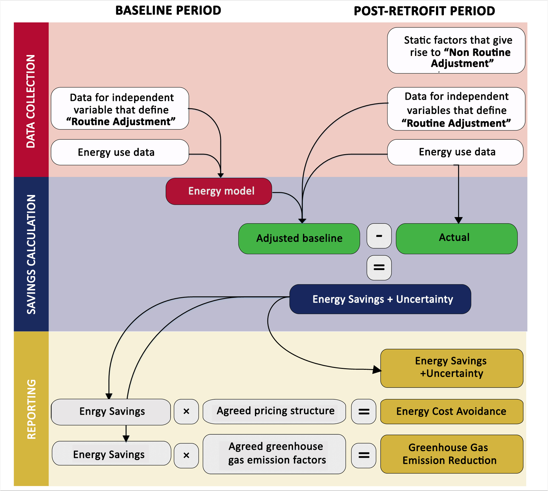
Since ESCOs should usually guarantee that the improvements will generate sufficient energy savings and hence relevant costs to pay for the project over the term of the contract, a mutually accepted M&V plan is inevitable based on which energy savings are quantified. In other words, since energy savings cannot be measured, one should establish Energy Baselines (EnBs) to compare energy consumption before and after the ECM implementation to calculate savings. See the process diagram of standard savings calculation below [1].
Figure 1- Process diagram of standard savings calculation
EnB establishment has a broad discussion that is beyond the scope of this article. Among all those issues, the selection of appropriate variables with respect to Significant Energy Uses (SEUs) and its statistical tests will be discussed here in the building sector.
Energy Baseline
An energy baseline reflects a specified period of time and is a quantitative reference providing a basis for comparison of energy performance between two periods called baseline period (before any ECM is implemented) and reporting period (after the ECM is commissioned), where variables affecting energy uses and/or consumption can be considered [2]. To follow the process of energy performance measurement using EnBs, once boundaries and energy flows are defined, M&V experts might prepare a list of possible variables through brainstorming, determine a suitable baseline period, gather data and try to test the relevance of each variable using regression and its statistical tests. These variables can be selected and the regression can be developed more appropriately when energy uses with their consumption shares are determined. Energy use refers to energy applications (such as lighting, heating, cooling, cooking, etc. in the building sector) and significant energy uses are the ones accounting for substantial energy consumption and/or offering considerable potential of improvement [3]. The former significance criterion is considered only in this article. This idea is discussed thoroughly below within a case study.
Case Study
Consider natural gas consumption in a complex of administrative buildings with a single supplier meter to measure energy consumption. To measure energy performance and establish the most appropriate EnB, suitable measurement boundaries should be defined initially. As the installed meter measures gas consumption of 5 separate buildings as well as a restaurant in whole, the complex forms the energy performance boundary. Once the boundary is defined, relevant variables that are likely to have an impact on energy consumption should be determined and quantified. It is important to isolate those variables which are significant in terms of energy performance from the variables which have little or no influence [2]. Some experts list all variables and use data analyses as well as statistical tests to determine these significant relevant variables. But once we know where and how energy is consumed in this boundary, it could be much easier to determine major variables according to the SEUs. Energy uses in this case is simulated accurately via Design Builder software based on detailed energy audit whose results are summarized below.
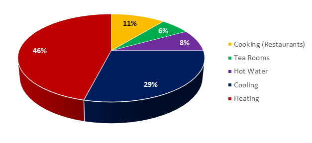
Table 1- Energy uses and their shares in NG consumption
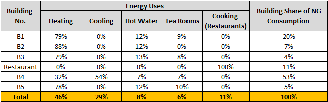
Figure 2- Summary of energy uses and their shares in NG consumption
Considering the SEUs in this case (heating and cooling respectively), HDD and CDD can be introduced as the major variables. The other energy uses can be considered either fixed in the form of the regression intercept (See Formula 1) or variable as a function of invoice period (See Formula 2).
Yi = a1 x HDD18,i + a2 x CDD21,i + b (1)
Yi = a1 x HDD18,i + a2 X CDD21,i + a3 x Periodi (2)
where:
Yi is natural gas consumption in each invoice (m3);
HDDi is heating degree days with a base temperature of 18oC calculated for each invoice (oC);
CDDi is cooling degree days with a base temperature of 21oC calculated for each invoice (oC);
Periodi is invoice period (days);
ai are the equation coefficients; and
b is the regression constant.
Detailed data analyses over three years reveals that invoice period does not vary markedly and has remained almost steady in the baseline period; i.e. the invoice periods all cover the range of their median value ± 10 days. Hence, this parameter can be considered fixed in this regression and the first formula seems appropriate. It should be noted that this is not true in all cases and invoice period can be a significant variable in some countries for the building sector depending on the frequency of meter readings (This can be discussed in another article). The regression results calculated by data analysis module in Excel software, is shown in Table 2 and discussed subsequently.
Table 2- NG regression summaries
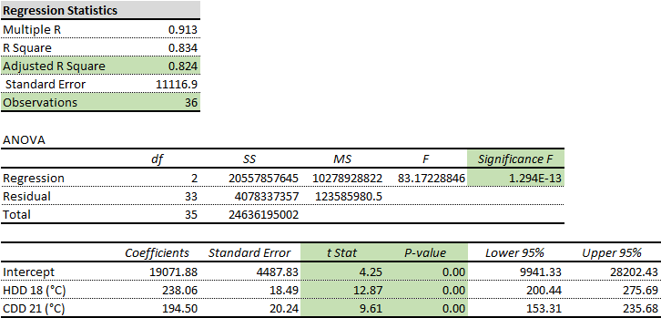
As data reveals, this regression passes the basic statistical tests including Adjusted R Square (greater than 0.75), Significance F (less than 0.05), and either t-Stat (greater than 2.035 that is calculated based on the model degree of freedom at confidence level of 95%) or P-values (less than 0.05) [See 4, clause 1.7. Modeling].
Besides, the coefficients sign and their minimum and maximum digits used in the regression shall be reviewed. In this regression, HDD and CDD both meet positive coefficients which can be interpreted as direct relationship between degree days and energy consumption, i.e. as degree-days increase (HDD in winters and CDD in summers), natural gas consumption boosts which seems definitely compatible with the building energy uses and trends. HDD and CDD both possess the minimum amount of zero in the baseline period, while the maximum amounts of 448.9 and 362.5 Celsius degrees are recorded respectively. This means that the equation is valid for these limits only; hence HDDs and/or CDDs in the reporting period with digits higher or lower than these amounts cannot be monitored using equation 1. The same is true about invoice period. Equation 1 is valid for the smallest and largest observations of invoice period in the baseline period, i.e. 20 and 39 days respectively.
So far, one might conclude that the model is accurate. This is not sufficient to accept or reject a statistical model, however, and more analyses is required as below. First, the RMSE or CV of the statistical model shall be determined. This can be calculated when the regression standard error (11,117 m3 in the preceding table) is divided by average NG consumption [See 4, clause 1.8. Modeling Errors]. The model CV is 16% which can arise from different sources including measurement, and statistical modeling. Simply put, when the CV formula is considered, the major factor that can affect its value is the residual of regression. A residual is the vertical distance between a data point and the regression line. In other words, to find the residual one would subtract the predicted value (Ŷi) from the measured value (Yi) for each x-value. Hence, both regression and measurement can rise total uncertainties and CV. Typically allthese different uncertainties are independent of each other and will be studied separately.
A) Measurement uncertainties
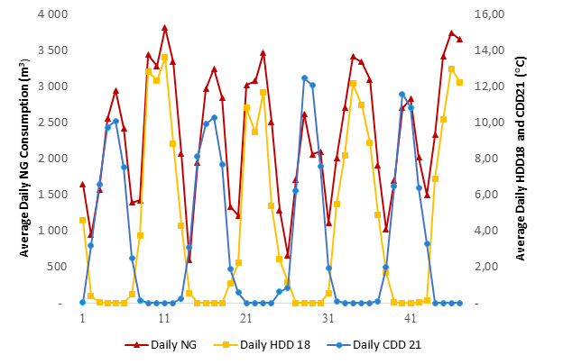
In most cases, we more or less assume that the measurement error is very small compared to the modeling error, especially if metering is relied on a revenue-grade meter, and hence this error is usually ignored. But this might not be true in all cases and shall be tested before any decision is made. The meter error can be reviewed and analyzed using relative as well as absolute precision calculated as 8998 m3 and 13% respectively in this case [See 4, clause 1.4.2. Confidence and Precision]. Furthermore, measurement data validation compared to major variables is studied in Figure 3, which reveals that NG consumption does not follow the buildings heating and cooling loads in some invoice periods and must end into higher modeling errors for those periods including numbers 2, 14, 26 and 29 in Table 3. Although, these periods can be labelled as outliers, data removal was impossible and forbidden in this case due to the fact that no reliable records of the complex history were known by the M&V experts.
Figure 3- Measurement data validation and error identification
B) Statistical errors
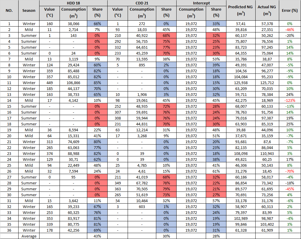
Once the model is developed and the coefficients are determined, the share of each variable in total predicts can be calculated and compared to the simulation results. As Table 3 suggests, the average share of HDD and CDD in predicted NG consumption is 43% and 30% respectively, which is relatively compatible with the simulation shares, i.e. 46% and 29% respectively. This can confirm the accuracy of the statistical modeling.
Table 3 - Calculation of variables share in total NG predicts
ENDNOTES
[1] Measurement and Verification Operational Guide, Office of Environment and Heritage NSW, Dec 2012
[2] ISO 50006:2014, Energy management systems- Energy performance measurement using energy baseline and energy performance indicators
[3] ISO 50001:2018, Energy management system- Requirements with guidance for use
[4] Uncertainty Assessment for IPMVP, July 2019

(*) This article produced under Consortio Limited, United Kingdom.