
![]() By Greg Anderson*
By Greg Anderson*
Monthly changes in building relative occupancy - percent of space leased - can greatly affect energy use in large commercial buildings, and especially in multi-tenant office buildings. Our experience performing measurement and verification of energy savings in real-world buildings suggests that using a baseline period longer than 12 months can offer improvements in reliability when quantifying occupancy impact.
When using IPMVP Option C, occupancy effects can be accounted for in the baseline model, rather than as non-routine events (NRE). If occupancy changes are present in the baseline period data, best practices suggest we should fit a secondary model of the residuals against relative occupancy to assess the statistical significance of the changes. If the occupancy term is significant, we include it in the baseline model either as an additional term or by separately applying the coefficient of the residual model to the predicted values of the baseline model (Koran and Rushton [1]).
However, there are situations where this approach may not work well. A worst-case scenario is a building where relative occupancy is nearly constant throughout the baseline period, so this factor is not included in the baseline model. We then observe a large occupancy change during the program assessment period. Non-routine event diagnostics flag a statistically significant change event around the same time. What do we do then?
A more subtle problem is that not all occupancy changes are equal on a per leased square foot basis. IT development firms and medical laboratories will have much higher plug load requirements than a sales office. Tenants will vary in their operating schedules, the number of employees per square foot, and their level of commitment to energy efficiency. These factors are impossible to capture in a model.
These problems, along with some possible remedies, are illustrated in the following real-world examples.
Let’s start with a straightforward case. Here we have almost two years of occupancy and interval data. Relative occupancy begins near 90% in early 2017 and then drops to just above 40% in late 2017 before rising back up to 55% in the spring of 2018.
Chart 1
A near-perfect relationship between occupancy and use.
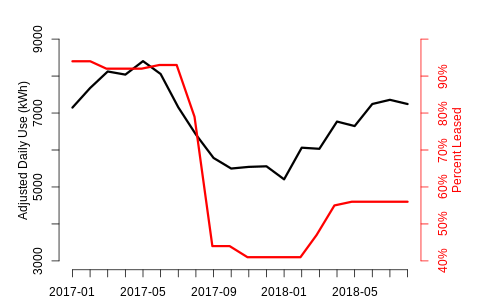
The use data is adjusted for weather. We fit a temperature and time of day model to remove weather effects and calculate average temperature-adjusted daily total use by month. The adjusted use vs occupancy correlation is high (.87) so we should be able to derive a reasonable estimate of the average impact of occupancy changes using this data.
Life is not always so kind to modelers however. In addition to the variation between tenants discussed above, occupancy values themselves are subject to random measurement errors. The resulting uncertainty is compounded by the fact that we have relatively few monthly observations to work with. We see an indication of this response variability in the chart below.
Chart 2
Why doesn’t use rebound to 2017 levels when occupancy does?
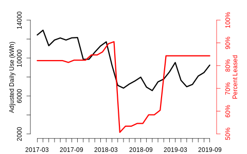
The large drop in occupancy in mid-2018 leads to an immediate drop in (temperature-adjusted) daily use, but when occupancy rebounds in 2019, energy use does not follow. A statistical change point algorithm [2] flags a potential non-routine event on April 13, 2018, suggesting the tenant moved out slightly earlier than the occupancy data indicates (occupancy is rarely tracked with greater than monthly granularity). The same algorithm shows no significant uptick around the time of the subsequent occupancy increase. Other factors may be at work here, but it does seem the new tenant had a minimal impact.
In practice a given building may see only a limited number of occupancy changes in any given 12-month period. What if those observed changes are atypical? Without an informative training data set, how can we make appropriate savings adjustments in the reporting period?
One obvious tack is to look at longer baseline periods. Multi-year series offer the potential for richer, more informative datasets to estimate occupancy effects. Below is an example of a three-year series.
Chart 3
A long time series with high natural variability is a best case scenario for a modeler

The length of this time series combined with its relatively large range of observed values bodes well for our ability to produce a reasonable estimate of occupancy effects. In fact, if we model temperature adjusted use against this occupancy series we get a highly statistically significant result.
Still, if you examine the chart above, you see periods of time where changes in occupancy are accompanied by varying response in adjusted use. We can formalize this observation by fitting rolling twelve-month models against this series. We end up with 28 coefficients, one for each twelve-month model. Here is the distribution of these results.
Chart 4
Occupancy elasticity varies widely using different 12 month rolling windows
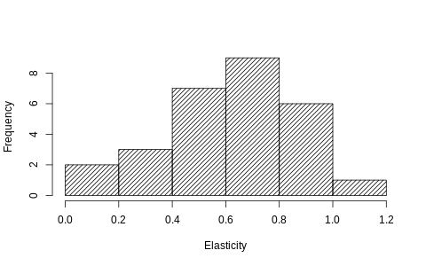
This example uses an elasticity model, where the log of adjusted use is regressed on the log of relative occupancy. This results in a dimensionless coefficient, not dependent upon the average level of usage in the training data, and allows for comparison of coefficients across different training sets and even buildings.
For comparison, the elasticity coefficient we get by fitting all of the available data is 0.57 with a 95% confidence interval of (0.51, 0.62); the mean of the rolling 12-month models (0.61) is near the upper end of the confidence interval. More concerning are the tail values, which range from 0.11 to 1.07. Depending on the twelve-month subsample chosen, the resulting elasticity could result in an implausibly high or low value.
This brings us back to our earlier “worst case” scenario where relative occupancy was nearly constant throughout the baseline period but we subsequently observe an occupancy change during the program assessment period. If we have pre-baseline occupancy data, we may be able to construct a reasonable occupancy adjustment using a longer-term data horizon.
Baseline models use twelve-month training periods to minimize contamination by NREs, but when attempting to estimate occupancy effects (and possibly other types of non-weather drivers, such as factory production data) longer series hold the promise of better estimates. This increases our chances of modeling a more representative mix of tenant changes - sales teams and IT firms - and also a wider range of occupancy values.
Of course, care must also be taken when drawing inferences from these longer, older, time series. Significant NREs could confound the occupancy effects. Historical data collection can be complicated by change in ownership or management staff turnover, and even recent data may not be of sufficiently high quality for our use. (A solid data collection strategy should be part of the M&V plan, but little can be done about poor historical data.) Still, the odds of producing a high-quality relative occupancy estimate seem enhanced if we have multiple years of observed effects available for consideration.
A good non-routine event detection algorithm used in conjunction with continuous monitoring of occupancy or other energy use drivers enhances the power of both sources of information. When we see coincident signals in both, we can have greater confidence that an event requires our attention.
Finally, in my ideal M&V world, modelers would have access to a rigorously collected and representative normative data set of comparative occupancy (and other) data. This would allow for, at a minimum, a head check for any values derived for a specific project. We might consider using this data as a proxy in situations where project-specific occupancy fails to produce a reasonable estimate, and we could possibly use this data as a source of priors in a Bayesian estimation framework. The collection of quality occupancy data for a single project can be time-consuming and difficult, so the assembling of a robust data set would be a large undertaking, but one can dream.
REFERENCES
[1] Reliability of Energy Savings Estimates Based onCommercial Whole Building Data. Prepared for the Regional Technical Forum, by Bill Koran and Josh Rushton, May 21, 2019.
[2] https://github.com/LBNL-ETA/nre

(*) Greg Anderson is Director of Data Science at Gridium.
![]()