
By Agenor Garcia* and Bruce Rowse**
This paper aims to explore in detail the concept of the measurement boundary, and how this affects the identification of independent variables, static factors and interactive effects in an M&V project. We review the basic IPMVP concepts and definitions of the IPMVP (from IPMVP Core Concepts, 2016), which, if incorrectly applied, can lead to various problems.
As examples of the problems that may arise we discuss one case using option C, and another example about the replacement of a chiller, which in the CMVP course is presented as a detailed example of both options A and B. To respond to the question “what should be the measurement boundaries” we give the example of a chiller upgrade in a commercial building and the replacement of a steam boiler. Following this, we attempt to “model” the process for the establishment of the measurement boundary for an M&V project. Finally, we discuss an interesting example of the installation of a heat exchanger in an industrial furnace to reinforce the concepts presented.
1. What the IPMVP says
Chapter 3 of IPMVP Core Concepts, 2016 defines the measurement boundary as “notational boundaries drawn around equipment, systems or facilities to segregate those which are relevant to savings determination from those which are not.” It is understood that the boundary is like a geographical or physical one, separating the equipment that impacts on the energy conservation measure (ECM) from that equipment which doesn’t. The definitions of routine adjustment – “Individually engineered calculations to account for the expected change in energy consumption or demand due to changes in the independent variables within the measurement boundary” - and static factors – “those characteristics of a facility which affect energy consumption and demand, within the defined measurement boundary, that are not expected to change, and were therefore not included as independent variables” - concludes that the operating conditions, independent variables and static factors, must be considered only within the measurement boundary. On the other hand, the interactive effects – “energy impacts created by an energy conservation measure that cannot be measured within the measurement boundary” - are a consequence of the ECM’s impact extending beyond the boundary, that is, affecting other energy using systems outside of the boundary.
Section 5.1 of the IPMVP Core Concepts, about the measurement boundary, only looks at one side, the energy boundary, separating out retrofit isolation - options A and B - from whole facility options (C). Option D, used in the case that sufficient measurement data is unavailable, and based on an engineering simulation, can be used as both a retrofit isolation method and a whole facility method.
There is no discussion about the measurement of independent variables, which in reality form the “other side” of the boundary, and are related to the energy services delivered. Earlier versions of the IPMVP allocated the meter as the marker of the boundary, which is no longer mentioned (but still true).
Because the boundary definition is very generic, it can result in poor interpretations. It is necessary to develop a deeper understanding of the concepts associated with the measurement boundary in order to be able to make the correct adjustments in the comparison of baseline energy use with reporting period energy use.
2. Examples of the problem and a solution
The first case presented is for option C. As the boundary encompasses the whole installation, it can be concluded that there are no interactive effects, because interactive effects only occur outside the boundary. However, if we had, for an example, multiple electric ECMs in a building, including a lighting upgrade, and the conditioning of the building was provided by gas heaters, there would be the interactive effect of gas use increasing due to less heat being produced by the lighting. This effect is not measured by the electricity meter, so it must be accounted for as an interactive effect.
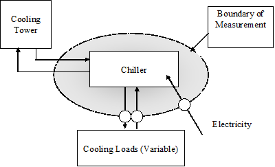
Figure 1 - Measurement boundary for a chiller replacement
Another problem of this imprecise definition can be seen in Module 7 - retrofit isolation details - of the CMVP training (see figure 1). In the example of option B, the replacement of a chiller is considered. Electrical energy supplied to the motor of the chiller and the thermal cooling load are correctly defined as the boundary with two limits, the energy supplied and the independent variable. The cooling tower is shown to be outside the boundary, because its parameters – entering condensing water temperature and the cooling towers themselves – are unchanged. None the less, in the CMVP training material says that “at least annually, review static factors to ensure baseline is still appropriate. E.g., cooling tower difficulties might have increased average condensing temperature.”
But, isn’t the cooling tower outside the measurement boundary? And aren’t the static factors obliged to be within the boundary? How do we resolve this problem?
In fact, as energy efficiency is about improving the efficiency of conversion of energy inputs to useful service outputs (such as lighting, cooling, etc), we should think about energy flows associated with the conversion of energy inputs into service outputs. So, we have two boundaries: one, on the side of the energy input, marked by the energy meter (for single measurements as well as for the whole installation) and another, on the side of the system output, the energy services, demand for which is correlated to the values of the independent variables. All the equipment and systems through which energy flows to deliver the services are within the measurement boundary and the rest are out. That is, we should think of the boundary not as a geographical boundary, such as the border of a country, but as a border of the flow of energy that provides the energy services that we are measuring.
In the example of Option C, the heat from lamps and ballasts leaves the measurement boundary because it is seen neither by the electricity meter nor by the meters of the independent variables (for example, external temperature and possibly occupancy). It is a genuine interactive effect, that is, an effect of the ECM that manifests itself in another energy system outside the measurement boundary because the boundary encompasses only the electricity use of the equipment.
In the example of the chiller, the cooling tower participates in the process of converting energy (from electricity to cold water) because the efficiency with which it cools the condensing water affects the performance of the chiller, since it affects the cooling of the refrigerant. For example, a loss in cooling capacity of the tower will impair refrigerant condensation and chiller operation. What is outside the measurement boundary is the energy expended by the tower in the fans and condensing water pumps, since only the electricity supplied to the chiller motor is being measured.
Thinking in terms of energy flow and the paths it takes to transform energy into services, we have a complete consideration of the boundary, that is, of independent variables, static factors and interactive effects. Let's look at some examples in more detail.
3. Other examples
3.1 Chiller in a shopping mall
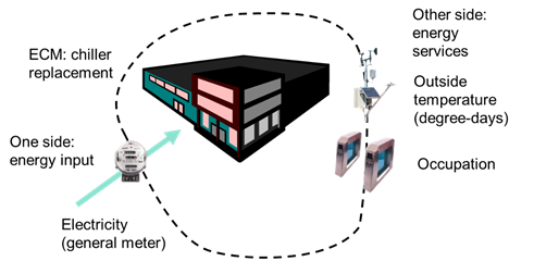
Figure 2 - Approach 1: Option C - Whole Facility
Let's go back to the chiller example, now in a specific installation - a shopping mall. Since air conditioning represents a large proportion of the consumption of electricity and chiller replacement has large energy savings, an option for M & V may be to use the mall's own electricity supply meter (which feeds the common areas) – i.e. Option C. Let’s assume that the independent variables are the external temperature (measured in degrees-day by means of data from a nearby meteorological station) and the occupancy of the mall (in people-days, measured by the shopping centre operator).
Electricity consumption measurements are made monthly by the electricity supplier. The measuring border, in this case, has one side defined by the energy meter of the electricity supplier and another by the whole installation, since any change in the structure of the mall (changes in number of stores, change of use in stores, etc.) is reflected in changes to the thermal load and chiller energy consumption.
In this configuration, the static factors include everything that happens inside the mall that affects energy consumption, except for the external temperature and occupancy. For example, lighting in common areas is a static factor and, if changed, needs a baseline adjustment (BLA). Any change in a store’s electricity usage changes the thermal load and also needs an BLA. It is therefore necessary to constantly monitor everything that happens within the electrical system of the common area and the thermal system of the whole mall (which can be a problem). A big advantage of this option is that the baseline (for example, the last 12 month’s consumption of electricity, temperature/degree days and occupancy) will probably be available.
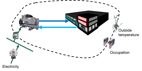
Figure 3 - Approach 2: Option A or B - Retrofit Isolation
If a large amount of BLAs are required, a solution may be to place an electricity meter on the power supply to the chiller, and use options A or B. The independent variables remain the external temperature and occupancy, because they significantly affect the consumption of the chiller. The difference is that the electrical system of the common areas is no longer a static factor, because it affects the overall site electricity meter, but not the chiller’s meter.
The major drawback is that if the meter is installed because of the ECM, you have to measure the entire baseline period. The IPMVP calls for a full cycle of the conditions of use, i.e. covering the entire spectrum of external temperature and occupancy, which can take a long time and delay the implementation of the ECM.
Static factor adjustments are only required where there are changes that impact on the thermal load of the air conditioning system, not changes to the electrical system (except where such changes may impact on the thermal load...). This is considered an Option B by the IPMVP (or A, depending on whether there are estimates or measurements of the key parameters).
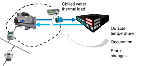
Figure 4 - Approach 3: Option A or B - Retrofit Isolation, with measurement of the thermal load
If static factors are challenging to keep track of, and require many BLAs, one can measure an intermediate variable defining the energy service, i.e. the thermal load of the chilled water.
The independent variable is now the thermal load itself. Daily or more frequent measurements may be used. The variation in external temperature and occupancy will be reflected in the thermal load and don’t need to be measured.
Also changes in the usage or size (i.e. number of shops) of the mall are reflected in the thermal load of the chilled water and do not represent a static factor. This solution is quite interesting as a measure of the improvement in conversion efficiency of the ECM itself, but it has a high measurement cost. It also doesn’t correlate the consumption with the conditions of use that mall owners would typically refer to, such as external temperature and occupancy. It is also necessary to measure the baseline before executing the ECM. This is also an IPMVP Option B (or A), since what defines the energy measurement boundary is only around the ECM and not the whole facility.
Table 1 below summarises the advantages and disadvantages of the three approaches presented below.
Table 1 - Advantages and disadvantages of the three approaches to M&V in the chiller example
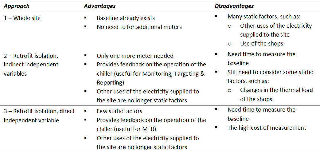
Approach 1 has a low cost of measurement, but there are many static factors that need to be monitored. Another advantage is that the variation in efficiency depends directly on variables already understood by the owner of the installation: temperature and occupancy.
Approach 2 is the middle ground between a wide boundary, linked to the usage of the mall, and a narrow one, linked to the performance of the chiller. Energy measurement is only for the chiller and the measurement of the independent variables comes from the wider boundary of the mall.
Approach 3 is focused on equipment performance. With meters installed, it can be used to track and optimize chiller performance through, for example, MT & R (Monitoring, Targeting and Reporting), using CUSUM (cumulative sum) techniques. It has a high cost of measurement, but does not require the monitoring of the conditions in the mall, which can be an advantage in environments which are changing.
3.2 Steam Boiler
Let's look at an example of M & V where the ECM is the replacement or an upgrade to a gas boiler that provides steam to an industrial facility, which may be manufacturing beverages, for example. Natural gas is used, in addition to the boiler feed, in some production furnaces. Some condensate is reused.
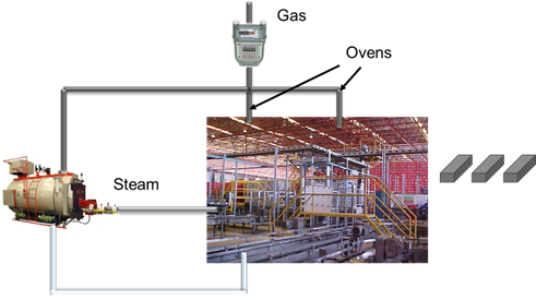
Figure 5 - Boiler replacement/upgrade ECM
The first approach would be to use gas utility measurements, probably correlated with factory output, which would explain most of the variation in gas consumption. Here we have a very large boundary, both for energy and the energy services, encompass the whole factory. Ovens would be static factors, because they use gas, in addition to the steam system. This approach is interesting because the baseline is ready, does not use additional measurement and correlates the gas consumption with variables which are important to the owner of the facility.
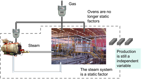
Figure 6 - Approach 2 for the boiler upgrade
If the ovens are not routinely used, requiring many BLAs, it is possible to install a gas meter exclusively on the gas supply to the boiler, still correlating gas consumption with factory production. Here the baseline should be measured, at points representative of the range in production variation, to have a good baseline model. Once the baseline is established and the ECM is implemented, IPMVP option B is the most appropriate because it will also allow monitoring and optimization of boiler performance. The ovens are no longer static factors, because they do not influence the boiler gas meter and are outside the measurement boundary. The steam system remains a static factor - changes in insulation of steam lines, changes to steam traps or their maintenance, and condensate recovery can change the steam / production ratio and thus require baseline adjustments.
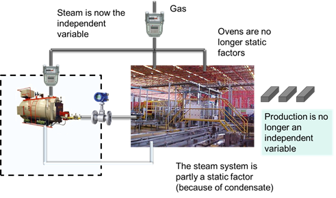
Figure 7 - Approach 3 for the boiler upgrade
The third option would be to measure the steam production along with the gas consumption. The boundary is restricted to the equipment and everything that happens in the factory and changes in the use of steam will already be detected by the steam meter. Production is no longer an independent variable and ovens are no longer static factors. The steam system is only a static factor if it affects the return of condensate. For example, if there was no return of condensate in the baseline period and condensate recovery was installed during the reporting period, there would be additional savings from condensate return and a BLA would have to be made. Here the concept of energy flow for defining the measurement boundary is clear - the return of condensate is within the boundary because it affects the efficiency of the boiler. It is a very useful option for the monitoring and optimization of boiler performance, but it has a high measurement cost.
[END OF PART I. - PART II WILL BE PUBLISHED IN THE DECEMBER 2018 ISSUE OF M&V FOCUS]
REFERENCES
EVO – Efficiency Valuation Organisation. Core Concepts, International Performance Measurement and Verification Protocol, 2016.
GERBI – Greenhouse gas Emissions Reduction in Brazilian Industry. M&V Case Study: Heat Recovery in a Furnace, power point presentation, Rio de Janeiro, 2003. Based on a problem initially proposed by John Cowan.

(*) Agenor Garcia is an energy efficiency and M&V consultant based in Brazil, technical director of CTC Experts. Agenor is a member of EVO's Extended Training Committee and an EVO L3 accredited instructor.

(**) Bruce Rowse is a consultant with 8020Green and is based in Australia. Bruce is the chairman of EVO's Extended Training Committee and an EVO L3 accredited instructor.